Timeseries at points
In this example. we will generate a GeoDataFrame with airport names and their coordinates. We will use those points to build a timeseries of precipitation at those locations.
First, we import emaremes and geopandas to build our GeoDataFrame.
[1]:
import geopandas as gpd
from pandas import Timestamp, Timedelta
from shapely.geometry import Point

import emaremes as mrms
Then, fetch hourly precipitation data for on the days during Hurricaine Helene:
[2]:
mrms.fetch.path_config.set_prefered("./data")

gribfiles = mrms.fetch.timerange(
    Timestamp("2024-09-26T12:00:00"),
    Timestamp("2024-09-28T00:00:00"),
    frequency=Timedelta(minutes=60),
)
Prefered path to store *new* Gribfiles is data
Now, let’s create a geodataframe with three airports:
[3]:
airports = {
    "Asheville Regional Airport": Point(-82.541, 35.436),
    "Jacksonville International Airport": Point(-81.689, 30.494),
    "Hartsfield-Jackson Atlanta International Airport": Point(-84.428, 33.641),
}

# Create a GeoDataFrame
gdf = gpd.GeoDataFrame(airports.keys(), geometry=list(airports.values()), columns=["Airport Name"], crs="EPSG:4326")

gdf["Code"] = ["AVL", "JAX", "ATL"]

gdf
[3]:
| Airport Name | geometry | Code | |
|---|---|---|---|
| 0 | Asheville Regional Airport | POINT (-82.541 35.436) | AVL |
| 1 | Jacksonville International Airport | POINT (-81.689 30.494) | JAX |
| 2 | Hartsfield-Jackson Atlanta International Airport | POINT (-84.428 33.641) | ATL |
We can use the explore method in geopandas to display a map of the data.
[ ]:
gdf.explore(column="Airport Name", categorical=True, zoom_start=7, cmap="Dark2", marker_kwds={"radius": 10})
To generate a timeseries in points, we use the ts.point module. For a single time step, a single MRMS GRIB file is queried, which returns a tuple with the datetime and the value at the points.
[5]:
mrms.ts.point.query_single_file(gribfiles[0], gdf.set_index("Code"))
[5]:
(np.datetime64('2024-09-26T16:00:00.000000000'),
 {'AVL': 1.5, 'JAX': 0.0, 'ATL': 4.300000190734863})
That is basically the building block to generate a timeseries. Passing the list of files to ts.point.query_files, emaremes will parallelize the process of opening each dataset and querying the points. This function will return a pandas dataframe with the data for each point.
[6]:
df = mrms.ts.point.query_files(gribfiles, gdf.set_index("Code"))
df
[6]:
| AVL | JAX | ATL | |
|---|---|---|---|
| timestamp | |||
| 2024-09-26 12:00:00+00:00 | 29.0 | 0.0 | 3.600000 |
| 2024-09-26 13:00:00+00:00 | 4.3 | 0.0 | 0.500000 |
| 2024-09-26 14:00:00+00:00 | 1.6 | 0.0 | 0.400000 |
| 2024-09-26 15:00:00+00:00 | 0.9 | 0.0 | 0.600000 |
| 2024-09-26 16:00:00+00:00 | 1.5 | 0.0 | 4.300000 |
| 2024-09-26 17:00:00+00:00 | 1.5 | 0.0 | 1.900000 |
| 2024-09-26 18:00:00+00:00 | 1.8 | 0.0 | 2.600000 |
| 2024-09-26 19:00:00+00:00 | 4.5 | 0.0 | 16.600000 |
| 2024-09-26 20:00:00+00:00 | 0.5 | 0.0 | 2.900000 |
| 2024-09-26 21:00:00+00:00 | 2.3 | 0.0 | 6.500000 |
| 2024-09-26 22:00:00+00:00 | 1.1 | 0.0 | 7.900000 |
| 2024-09-26 23:00:00+00:00 | 1.5 | 3.4 | 6.300000 |
| 2024-09-27 00:00:00+00:00 | 1.3 | 0.0 | 8.500000 |
| 2024-09-27 01:00:00+00:00 | 3.6 | 0.4 | 37.500000 |
| 2024-09-27 02:00:00+00:00 | 0.0 | 1.3 | 1.700000 |
| 2024-09-27 03:00:00+00:00 | 8.0 | 0.0 | 7.500000 |
| 2024-09-27 04:00:00+00:00 | 1.7 | 0.2 | 23.000000 |
| 2024-09-27 05:00:00+00:00 | 4.7 | 0.3 | 4.300000 |
| 2024-09-27 06:00:00+00:00 | 2.6 | 0.0 | 3.400000 |
| 2024-09-27 07:00:00+00:00 | 3.3 | 0.6 | 0.000000 |
| 2024-09-27 08:00:00+00:00 | 4.9 | 0.0 | 0.700000 |
| 2024-09-27 09:00:00+00:00 | 9.6 | 0.0 | 56.099998 |
| 2024-09-27 10:00:00+00:00 | 14.0 | 0.0 | 33.000000 |
| 2024-09-27 11:00:00+00:00 | 9.0 | 0.0 | 14.800000 |
| 2024-09-27 12:00:00+00:00 | 10.7 | 0.0 | 4.400000 |
| 2024-09-27 13:00:00+00:00 | 12.0 | 0.0 | 0.000000 |
| 2024-09-27 14:00:00+00:00 | 0.6 | 0.0 | 0.000000 |
| 2024-09-27 15:00:00+00:00 | 2.0 | 0.0 | 0.000000 |
| 2024-09-27 16:00:00+00:00 | 0.0 | 0.0 | 0.000000 |
| 2024-09-27 17:00:00+00:00 | 0.0 | 0.0 | 0.000000 |
| 2024-09-27 18:00:00+00:00 | 0.0 | 0.0 | 0.000000 |
| 2024-09-27 19:00:00+00:00 | 0.0 | 0.0 | 0.000000 |
| 2024-09-27 20:00:00+00:00 | 0.0 | 0.0 | 0.000000 |
| 2024-09-27 21:00:00+00:00 | 0.0 | 0.0 | 0.000000 |
| 2024-09-27 22:00:00+00:00 | 0.0 | 0.0 | 0.000000 |
| 2024-09-27 23:00:00+00:00 | 0.0 | 0.0 | 0.000000 |
| 2024-09-28 00:00:00+00:00 | 0.0 | 0.0 | 0.000000 |
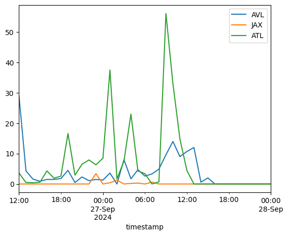
Notice that the column names of the retuned dataframe are the index in the geodataframe.
[7]:
df.plot()
[7]:
<Axes: xlabel='timestamp'>