Timeseries at polygons
This notebook shows how to extract precipitation rate timeseries from MRMS GRIB2 files for specific geographical areas.
[1]:
import geopandas as gpd
from shapely.geometry import Polygon
from pandas import Timestamp, Timedelta

import emaremes as mrms
First, we download hourly precipitation rate data during Hurricane Helene in September 2024:
[2]:
mrms.fetch.path_config.set_prefered("./data")

gribfiles = mrms.fetch.timerange(
    Timestamp("2024-09-26T12:00:00"),
    Timestamp("2024-09-28T00:00:00"),
    frequency=Timedelta(minutes=60),
)
Prefered path to store *new* Gribfiles is data
We define three rectangular polygons spanning different latitudes to analyze precipitation patterns:
Rect_0: 38°N-40°N, 85°W-83°W
Rect_1: 35°N-37°N, 85°W-83°W
Rect_2: 32°N-34°N, 85°W-83°W
[3]:
polygons = {
    "Rect_0": Polygon.from_bounds(-85, 38, -83, 40),
    "Rect_1": Polygon.from_bounds(-85, 35, -83, 37),
    "Rect_2": Polygon.from_bounds(-85, 32, -83, 34),
}

gdf = gpd.GeoDataFrame(polygons.keys(), geometry=list(polygons.values()), columns=["Rect"], crs="EPSG:4326")
gdf
[3]:
| Rect | geometry | |
|---|---|---|
| 0 | Rect_0 | POLYGON ((-85 38, -85 40, -83 40, -83 38, -85 ... |
| 1 | Rect_1 | POLYGON ((-85 35, -85 37, -83 37, -83 35, -85 ... |
| 2 | Rect_2 | POLYGON ((-85 32, -85 34, -83 34, -83 32, -85 ... |
The polygons are plotted on a map to show their geographical locations, using the explore method of the GeoDataFrame.
[4]:
gdf.explore(
    column="Rect",
    categorical=True,
    zoom_start=5,
    cmap="Dark2",
)
[4]:
Extract timeseries
We can extract precipitation rate values for each polygon:
From a single file (one timestamp)
From all files to create a complete timeseries
For a single file, we obtain a tuple with the timestamp and the mean precipitation rate values:
[5]:
mrms.ts.polygon.query_single_file(gribfiles[23], gdf.set_index("Rect"))
[5]:
(np.datetime64('2024-09-27T11:00:00.000000000'),
 {'Rect_0': 1.7448673248291016,
  'Rect_1': 2.15366268157959,
  'Rect_2': 3.3074347972869873})
This same could have been done with xarray’s open_dataset function. For multiple times, we could use xr.open_mfdataset and concatenate the GRIB files in the date dimension. However, for a large number of timesteps, this is slower than using ts.polygon.query_files.
[6]:
df = mrms.ts.polygon.query_files(gribfiles, gdf.set_index("Rect"))
df
[6]:
| Rect_0 | Rect_1 | Rect_2 | |
|---|---|---|---|
| timestamp | |||
| 2024-09-26 12:00:00+00:00 | 0.025535 | 2.004335 | 3.394098 |
| 2024-09-26 13:00:00+00:00 | 0.050047 | 2.336812 | 3.984890 |
| 2024-09-26 14:00:00+00:00 | 0.054240 | 2.450260 | 3.343230 |
| 2024-09-26 15:00:00+00:00 | 0.167617 | 2.070517 | 3.131488 |
| 2024-09-26 16:00:00+00:00 | 0.321593 | 1.784028 | 3.234480 |
| 2024-09-26 17:00:00+00:00 | 0.316905 | 1.604585 | 3.798618 |
| 2024-09-26 18:00:00+00:00 | 0.217352 | 1.431217 | 4.528488 |
| 2024-09-26 19:00:00+00:00 | 0.164745 | 1.511670 | 5.032995 |
| 2024-09-26 20:00:00+00:00 | 0.264327 | 1.903472 | 4.187413 |
| 2024-09-26 21:00:00+00:00 | 0.294353 | 2.089133 | 4.942948 |
| 2024-09-26 22:00:00+00:00 | 0.175707 | 2.146783 | 4.570075 |
| 2024-09-26 23:00:00+00:00 | 0.121927 | 2.146390 | 3.430357 |
| 2024-09-27 00:00:00+00:00 | 0.214432 | 2.081162 | 3.747465 |
| 2024-09-27 01:00:00+00:00 | 0.261622 | 2.526337 | 5.651672 |
| 2024-09-27 02:00:00+00:00 | 0.379312 | 2.182310 | 4.780615 |
| 2024-09-27 03:00:00+00:00 | 0.604708 | 2.545425 | 6.274500 |
| 2024-09-27 04:00:00+00:00 | 0.746275 | 2.696373 | 5.673342 |
| 2024-09-27 05:00:00+00:00 | 0.753362 | 2.923440 | 5.875688 |
| 2024-09-27 06:00:00+00:00 | 0.892322 | 3.068248 | 7.670566 |
| 2024-09-27 07:00:00+00:00 | 1.558730 | 2.773507 | 9.282417 |
| 2024-09-27 08:00:00+00:00 | 2.182055 | 2.548048 | 7.422433 |
| 2024-09-27 09:00:00+00:00 | 1.832045 | 3.379890 | 6.314767 |
| 2024-09-27 10:00:00+00:00 | 1.671623 | 2.580290 | 4.750607 |
| 2024-09-27 11:00:00+00:00 | 1.744867 | 2.153663 | 3.307435 |
| 2024-09-27 12:00:00+00:00 | 1.791805 | 2.890290 | 0.829160 |
| 2024-09-27 13:00:00+00:00 | 2.051350 | 2.705640 | 0.091732 |
| 2024-09-27 14:00:00+00:00 | 2.205035 | 2.235087 | 0.012025 |
| 2024-09-27 15:00:00+00:00 | 2.141853 | 1.209677 | 0.000000 |
| 2024-09-27 16:00:00+00:00 | 4.006072 | 0.528278 | 0.000458 |
| 2024-09-27 17:00:00+00:00 | 4.899700 | 0.447050 | 0.001175 |
| 2024-09-27 18:00:00+00:00 | 5.279102 | 0.218468 | 0.000000 |
| 2024-09-27 19:00:00+00:00 | 6.793183 | 0.120420 | 0.000000 |
| 2024-09-27 20:00:00+00:00 | 3.619245 | 0.033625 | 0.000000 |
| 2024-09-27 21:00:00+00:00 | 4.593427 | 0.016060 | 0.000000 |
| 2024-09-27 22:00:00+00:00 | 3.091657 | 0.000648 | 0.000000 |
| 2024-09-27 23:00:00+00:00 | 2.426183 | 0.001717 | 0.000000 |
| 2024-09-28 00:00:00+00:00 | 1.663122 | 0.013210 | 0.000000 |
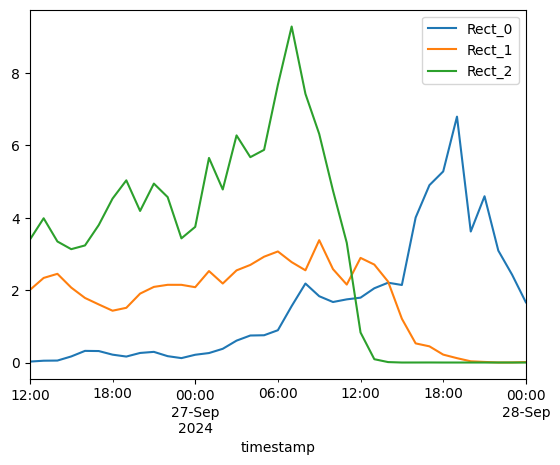
[7]:
df.plot()
[7]:
<Axes: xlabel='timestamp'>